All You Need To Know About Merging (Joining) Datasets in R
This article is also available in Spanish.
Merging—also known as joining—two datasets by one or more common ID variables (keys) is a common task for any data scientist. If you get the merge wrong you can create some serious damage to your downstream analysis so you’d better make sure you’re doing the right thing! In order to do so, I’ll walk you through three different approaches to joining tables in R: the {base} way, the {dplyr} way and the SQL way (yes, you can use SQL in R).
Types of Merges
First of, though, let’s review the different ways you can merge datasets. Borrowing from the SQL terminology I will cover these four types:
- Left join
- Right join
- Inner join
- Full join
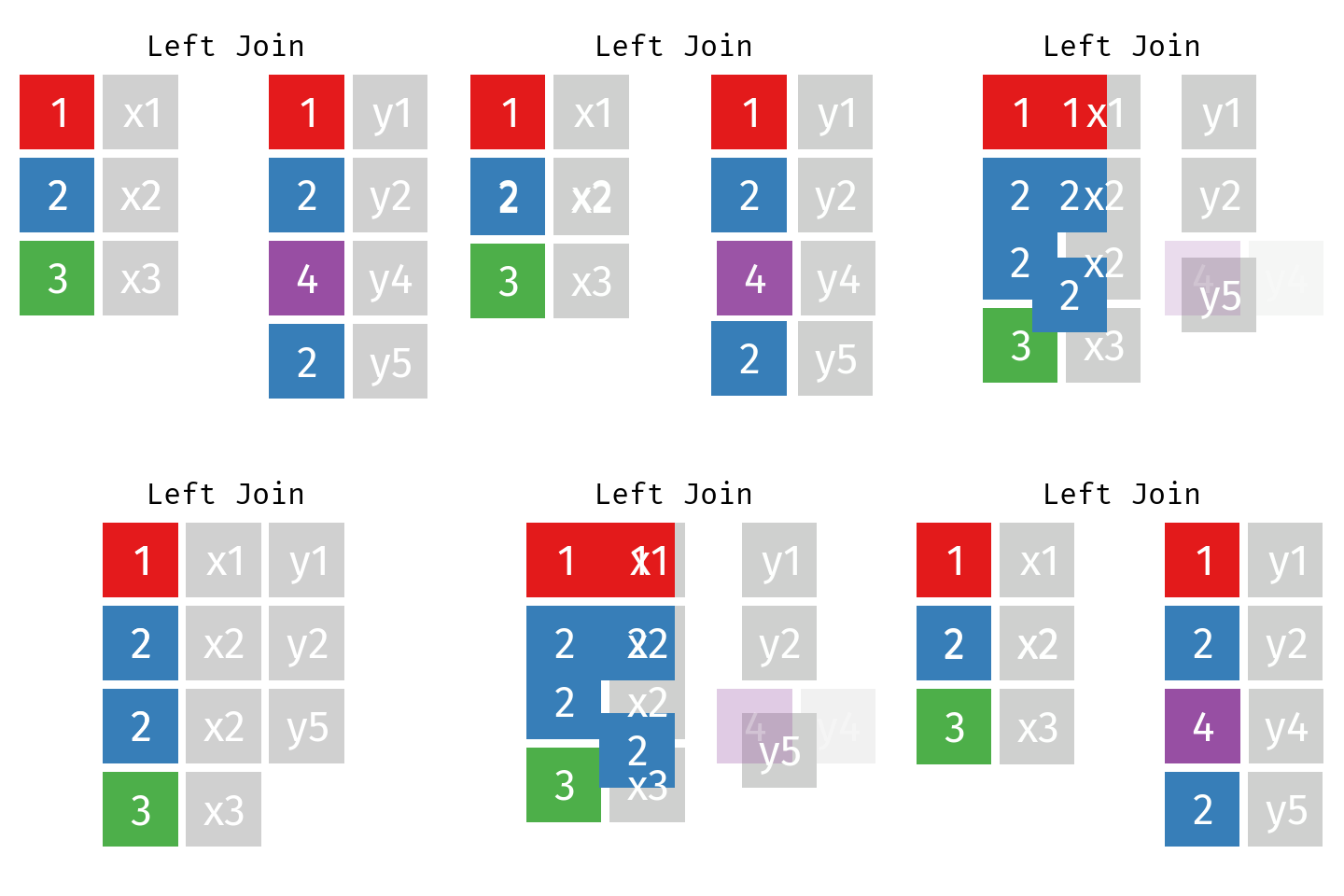
Left Join
In a left join involving datasets L and R the final table—let’s call it LR—will contain all records from dataset L but only those records from dataset R whose key (ID) is contained in L.

Right Join
A right join is just like a left join but the other way around: the final table contains all rows from R and only those from L with a matching key. Note that you can re-write any right join of L with R as a left join of R with L.

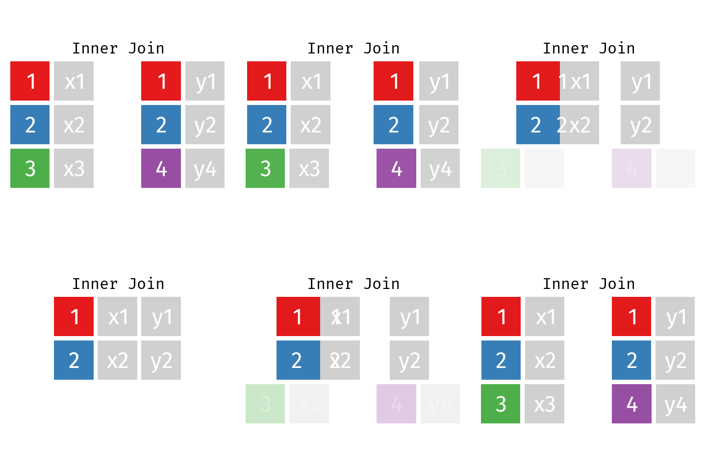
Inner Join
In an inner join only those records from L and R who have a matching key in the other dataset are contained in the final table.

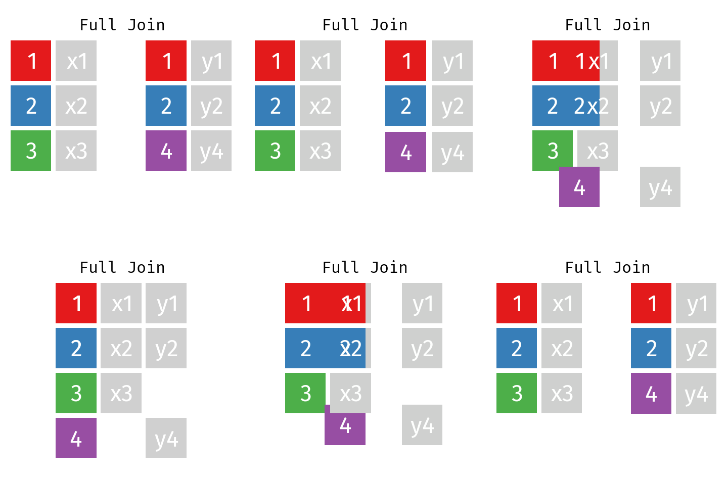
Full Join
By using a full join the resulting dataset contains all rows from L and all rows from R regardless of whether or not there’s a matching key.

The {base} Way
Enough of the theory, let’s explore how to actually perform a merge in R. First of, the {base} way. In {base} R you use a single function to perform all merge types covered above. Conveniently, it is called merge().
To illustrate the concepts I will use two fictitious datasets of a clinical trial. One table contains demographic information and the other one adverse events recorded throughout the course of the trial. Note that patient P2 has a record in demographics but not in adverse_events and that P4 is contained in adverse_events but not in demographics.
demographics <- data.frame(
  id = c("P1", "P2", "P3"),
  age = c(40, 54, 47),
  country = c("GER", "JPN", "BRA"),
  stringsAsFactors = FALSE
)
adverse_events <- data.frame(
  id = c("P1", "P1", "P3", "P4"),
  term = c("Headache", "Neutropenia", "Constipation", "Tachycardia"),
  onset_date = c("2020-12-03", "2021-01-03", "2020-11-29", "2021-01-27"),
  stringsAsFactors = FALSE
)
By default, merge() will perform an inner join: only those patients that appear in both the demographics and adverse_events datasets are included in the final table.
merge(
  x = demographics,
  y = adverse_events,
  by = "id"
)
## id age country term onset_date
## 1 P1 40 GER Headache 2020-12-03
## 2 P1 40 GER Neutropenia 2021-01-03
## 3 P3 47 BRA Constipation 2020-11-29
To perform a left join, set the all.x parameter to TRUE. For a right join do the same with the all.y parameter.
merge(
  x = demographics,
  y = adverse_events,
  by = "id",
  all.x = TRUE
)
## id age country term onset_date
## 1 P1 40 GER Headache 2020-12-03
## 2 P1 40 GER Neutropenia 2021-01-03
## 3 P2 54 JPN <NA> <NA>
## 4 P3 47 BRA Constipation 2020-11-29
merge(
  x = demographics,
  y = adverse_events,
  by = "id",
  all.y = TRUE
)
## id age country term onset_date
## 1 P1 40 GER Headache 2020-12-03
## 2 P1 40 GER Neutropenia 2021-01-03
## 3 P3 47 BRA Constipation 2020-11-29
## 4 P4 NA <NA> Tachycardia 2021-01-27
Finally, a full join can be performed by either setting both all.x and all.y to TRUE or specifying all = TRUE.
merge(
  x = demographics,
  y = adverse_events,
  by = "id",
  all = TRUE
)
## id age country term onset_date
## 1 P1 40 GER Headache 2020-12-03
## 2 P1 40 GER Neutropenia 2021-01-03
## 3 P2 54 JPN <NA> <NA>
## 4 P3 47 BRA Constipation 2020-11-29
## 5 P4 NA <NA> Tachycardia 2021-01-27
In the two example datasets I created, the common key is conveniently called id in both tables. However, this doesn’t necessarily have to be the case. If the two datasets you’d like to merge have different names for their common ID variables you can specify them individually using the by.x and by.y parameters of merge().
adverse_events2 <- adverse_events
colnames(adverse_events2)[1L] <- "pat_id"
merge(
  x = demographics,
  y = adverse_events2,
  by.x = "id",
  by.y = "pat_id",
  all = TRUE
)
## id age country term onset_date
## 1 P1 40 GER Headache 2020-12-03
## 2 P1 40 GER Neutropenia 2021-01-03
## 3 P2 54 JPN <NA> <NA>
## 4 P3 47 BRA Constipation 2020-11-29
## 5 P4 NA <NA> Tachycardia 2021-01-27
The {dplyr} Way
Unlike {base} R—which uses a single function to perform the different merge types—{dplyr} provides one function for each type of join. And fortunately they are named just as you’d expect: left_join(), right_join(), inner_join() and full_join(). Personally I’m a big fan of this interface and thus tend to use {dplyr} for joining datasets much more often than {base}.
library(dplyr)
left_join(demographics, adverse_events, by = "id")
## id age country term onset_date
## 1 P1 40 GER Headache 2020-12-03
## 2 P1 40 GER Neutropenia 2021-01-03
## 3 P2 54 JPN <NA> <NA>
## 4 P3 47 BRA Constipation 2020-11-29
inner_join(demographics, adverse_events, by = "id")## id age country term onset_date
## 1 P1 40 GER Headache 2020-12-03
## 2 P1 40 GER Neutropenia 2021-01-03
## 3 P3 47 BRA Constipation 2020-11-29
full_join(demographics, adverse_events, by = "id")## id age country term onset_date
## 1 P1 40 GER Headache 2020-12-03
## 2 P1 40 GER Neutropenia 2021-01-03
## 3 P2 54 JPN <NA> <NA>
## 4 P3 47 BRA Constipation 2020-11-29
## 5 P4 NA <NA> Tachycardia 2021-01-27
In case the ID variable names of the two tables do not match you need to pass a named vector as argument to by. The name and value corresponds to the key in the first and second table, respectively.
right_join(demographics, adverse_events2, by = c("id" = "pat_id"))## id age country term onset_date
## 1 P1 40 GER Headache 2020-12-03
## 2 P1 40 GER Neutropenia 2021-01-03
## 3 P3 47 BRA Constipation 2020-11-29
## 4 P4 NA <NA> Tachycardia 2021-01-27
The SQL Way
When it comes to merging tables there’s no way one cannot mention the structured query language (SQL). There are several R packages available from CRAN to directly send SQL queries from R to a database. The {tidyquery} package does something different, though. It takes the SQL query you provide the query() function as input, translates it to {dplyr} code and then executes this {dplyr} code to produce the final result.
library(tidyquery)
query("select * from demographics right join adverse_events using(id)")
## id age country term onset_date
## 1 P1 40 GER Headache 2020-12-03
## 2 P1 40 GER Neutropenia 2021-01-03
## 3 P3 47 BRA Constipation 2020-11-29
## 4 P4 NA <NA> Tachycardia 2021-01-27
query("select * from demographics inner join adverse_events using(id)")## id age country term onset_date
## 1 P1 40 GER Headache 2020-12-03
## 2 P1 40 GER Neutropenia 2021-01-03
## 3 P3 47 BRA Constipation 2020-11-29
query("select * from demographics full join adverse_events using(id)")## id age country term onset_date
## 1 P1 40 GER Headache 2020-12-03
## 2 P1 40 GER Neutropenia 2021-01-03
## 3 P2 54 JPN <NA> <NA>
## 4 P3 47 BRA Constipation 2020-11-29
## 5 P4 NA <NA> Tachycardia 2021-01-27
For simple queries—like joining tables—this is probably overkill given {dplyr}’s interface is so similar to SQL. However, if you are a SQL wizard and write more complex queries, {tidyquery} can be a great way to become proficient in {dplyr} as it can actually show you the translated {dplyr} code.
show_dplyr("
  select dm.id, dm.age, ae.term
  from demographics as dm
  left join adverse_events as ae
  using(id)
  where term <> 'Headache'
")
## demographics %>%
## left_join(adverse_events, by = "id", suffix = c(".dm", ".ae"), na_matches = "never") %>%
## filter(term != "Headache") %>%
## select(id, age, term)
By the way, there’s also the {dbplyr} package which translates your {dplyr} code into SQL. That way you don’t actually need to learn SQL in order to query a database.
In this articles we’ve covered the four most common ways of joining tables and how to implement them in R using {base}, {dpyr} and SQL via {tidyquery}. Armed with this knowledge you should be able to confidently merge any datasets you come across in R. If you do get stuck feel free to ask a question in the comments below.